
Time Series - Basic concepts
In this post, let us explore the basic concepts about time series. We will also learn about resampling techniques, how to check for stationarity and ways to convert non stationary series into stationary series.
What is time series
In time series, data are recorded over time. Time interval may be daily, monthly, yearly etc.
How to import time series data
Refer the post Importing Time Series data into Python.
Handling missing values
Handling missing values post provides information on handling missing values. Depending upon the case, generally it is advisable to fill the missing values with previous value or next value or using interpolation techniques or moving averages or using time series models.
Resampling:
A) Downsampling
In simple terms, it is like aggregating. For example: converting daily data to monthly data, or quarterly data to yearly data etc.
In the following example, I have converted daily data to weekly data.
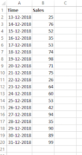
Original data
In resample option, use rule='W' for weekly frequency. Other commonly used rules are B (Business day), M (Monthly), A or Y (year end frequency). For more rules, you can refer this document.
In the below picture, not how changing the label='left' changes the week in resampled data3. We can aggregate the data using measures such as 'sum', 'mean' etc.

B) Upsampling

Original data

Upsampled data with 'bfill' method to handle empty values
Visualizing time series data
To plot:
plt.plot(data)
Stationarity
- Strict stationarity : all time series properties are time invariant.
- Weak (Wide-sense stationarity): mean, variance and autocorrelation are time invariant.
Why we need the series to be stationary
If we want to predict future, then if we fit a good model on stationary data, it will accurately predict the future as its statistical properties do no change over time.
How to test the stationarity
- Plots- Visualization will give a broad idea about trend, variation in the time series
- Augmented Dickey–Fuller test

Augmented Dickey–Fuller test
For this test, I have used the code from this blogpost and slightly modified it.
- Kwiatkowski-Phillips-Schmidt-Shin Test
In this test, unlike the ADF test, null hypothesis is series is stationary around a level or trend. Let us see how to run:
a) Null hypothesis that time series is level stationary

b) Null hypothesis that time series is trend stationary
Additionally use regression =’ct’ option to test trend stationarity.

KPSS test with Null hypothesis-trend stationarity
Phillips–Perron test can also be used to test stationarity.
How to convert non stationary series to stationary series
Commonly followed strategies are:
- Log transformation
Log transformation are commonly used in time series data. It is useful when the values are positive and exponentially growing.

- Differencing
First order differencing is generally sufficient to convert most of the time series data to stationary series.

- Seasonal differencing
In the following example, let us see how to difference the series (D), then perform seasonal differencing (d).

Now perform seasonal differencing (since this is the monthly data, 12 will be the order of seasonal differencing).

We can use any combinations of these transformations to transform the time series depending upon the situation.
White Noise
White noise is a series whose values are uncorrelated with zero mean and finite variance. We want the error terms of our model to be a white noise process. It is a stationary series.
Random walk
If an observation is dependent only on its previous value(as shown below), then that series is said to follow random walk.
Yt =Yt-1+Et
which is,
Yt -Yt-1 = Et (which means differenced series is white noise)
Another type of random walk model: random walk with drift (α).
Yt = α+Yt-1+Et
Yt -Yt-1 = α+Et (which means differenced series is equal to white noise + α)
One thing to note that while random walk series is non-stationary, not all non-stationary series follow random walk (more on this).
Summary
In this post, we have explored
- what is time series data
- resampling (downsampling and upsampling)
- stationarity-concept and tests
- differencing
- white noise
- random walk model


